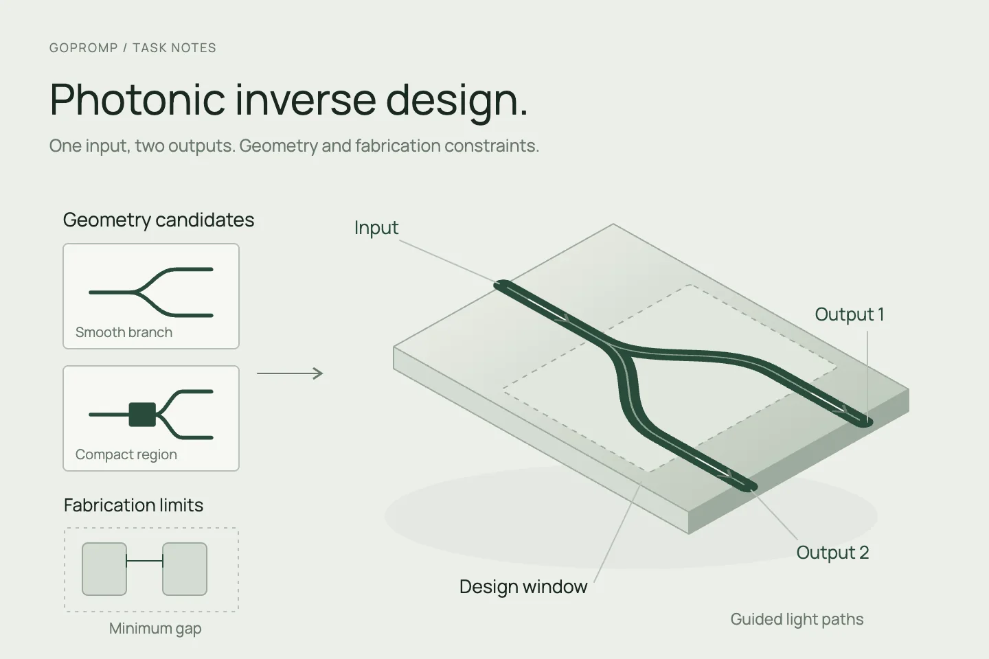
Sending input light into two waveguides at an agreed ratio on a photonic chip may seem like a simple splitting task. In practice, the design must also account for bandwidth, reflection, footprint and fabrication conditions. Similar power at both outputs does not necessarily mean good transmission: after a large input-power loss, the remaining outputs can still be well balanced.
For this kind of R&D task, we start with the port performance required by the circuit and organise geometric candidates, electromagnetic computation and checks around it. Optimisation determines how to change a structure; independent computation assesses whether the change holds up. Once fabrication and measurement are available, sample differences inform the next design round.
Task targets and broadband evaluation
First fix the material stack, waveguide interfaces, input mode and target polarisation. Define the operating band, splitting ratio, allowable loss and reflection. Save port reference positions with the task to avoid mixing propagation losses from connecting waveguides of different lengths into the device comparison.
Evaluation needs to consider power in the target output modes, the splitting ratio and input reflection together. Optimising only the ratio can reward candidates with poor transmission; a band-wide average can conceal failure at individual wavelengths. Set thresholds from usage requirements, examine the poorer parts of the band and retain the footprint–performance trade-off.
Initial optimisation can use representative wavelengths; validation should examine a denser spectrum and wavelengths not used for tuning. State the scope if only one polarisation is required. For dual polarisation, evaluate each input separately rather than extending results from one to the other.
Geometric candidates and fabrication constraints
We first establish an editable parametric baseline with variables such as branch shape, transition sections and local contours. The design space is smaller but easier to explain and modify. If these changes cannot meet the target, consider topology candidates that vary material distribution within a defined area, allowing holes, connections and boundaries to change together.
Continuous material weights in topology optimisation are a computational representation, not a fabrication layout. Candidates need material separation, contour extraction and dimensional checks for line widths, gaps, curvature and port continuity against the agreed process. Minimum-feature constraints must cover both material and voids. Remeasure the exported layout; the optimiser’s constraint values alone do not establish a pass.
These choices affect optical performance. Simply removing small holes or smoothing sharp corners late in the process can destroy the original response. Fabrication requirements should therefore enter candidate construction early, and the final exported geometry still needs new electromagnetic checks.
Adjoint optimisation and AI surrogates
The adjoint method uses forward and adjoint electromagnetic solves to obtain gradients of the objective with respect to design variables, helping an optimiser adjust many geometric degrees of freedom. It derives from physical equations and sensitivity analysis; it is not itself machine learning. Save the objective definition and gradient path, and check gradients with finite perturbations in selected directions to detect changes introduced by the geometry mapping.
It generally finds improvements near the current starting point; it does not prove a globally optimal structure. Compare multiple starting points or geometric representations using the same performance definitions.
If simulation data adequately covers the task range, an AI surrogate can estimate candidate spectra, screen starting structures or select designs worth detailed computation. Group training and held-out data by complete structures and their variants, and check prediction errors and validity range. Out-of-range candidates return to electromagnetic solves. With insufficient data, start with physics-based optimisation rather than spending the computation budget on training. Re-solve every final surrogate-recommended structure.
Independent electromagnetic checks and numerical convergence
Once a candidate is frozen, rebuild the checking model from the exported geometry and verify coordinates, material dispersion, layer thicknesses and port numbering. The checking workflow independently reads targets and results; optimiser-log scores do not stand in for validation.
Normalise input power at each wavelength and decompose output into the agreed waveguide modes. Port cross-sections should contain the mode field and distinguish propagation directions. Check the power balance among incident, reflected, output, radiated and absorbed power. Energy outside the target mode is not automatically material absorption. Field images locate phenomena; port power determines transmission performance.
Vary the mesh, absorbing-boundary distance and thickness, and run duration separately to test convergence of the quantities that matter. A 2D approximation can support screening, but candidates must be checked in the actual 3D layer stack for vertical radiation and mode differences. Where practical, cross-check key candidates using another discretisation or solver. If rankings change with these settings, resolve numerical or modelling causes before further structural optimisation.
Fabrication variation and measurement mismatch
Before fabrication, establish line-width bias, layer-thickness and sidewall variation conditions from process evidence and re-solve each candidate. Uniform contour expansion or contraction represents some systematic biases, not all edge roughness or local defects. Variation ranges need evidence; arbitrary perturbations do not establish fabrication robustness.
Sample measurements retain records of the device, reference waveguide, input polarisation, coupling and instrument calibration. Different coupling efficiencies at the outputs can distort the measured ratio; reduced reference-structure transmission can also affect device-loss estimates. Record repeated coupling measurements and measurements of different samples separately.
When measurement and prediction disagree, check references and calibration first. If the difference changes substantially with coupling adjustment, address the measurement path. If multiple samples show a consistent bias and calculations using measured geometry explain it, update the fabrication model and robust-design conditions. When the cause remains unclear, plan measurements that distinguish material, geometry and test effects instead of fitting all discrepancy into the surrogate.
Design revision and delivery
Each revision should identify whether it changes geometry, material assumptions, fabrication conditions or measurement processing. Re-export and check affected candidates and rerun previously passed checks. Evaluate the updated design using wavelengths, variation conditions or independent samples not used for tuning, retaining unexplained differences.
The interface is organised around design comparison. Users can open a candidate’s port spectra, process checks, solver settings and failures, then return to its original geometry version. Optimisation, independent computation and sample measurements appear separately so the team can decide which structures merit fabrication and which conditions need more evidence.
Delivery includes editable designs and layouts, computation and optimisation scripts, material and port configurations, independent-check records and a measurement plan. GOPROMP handles the agreed software and computation workflow and arranges fabrication and testing with customer teams that have the necessary facilities. Each conclusion states its checked level and scope, giving the next R&D round a specific difference to investigate.