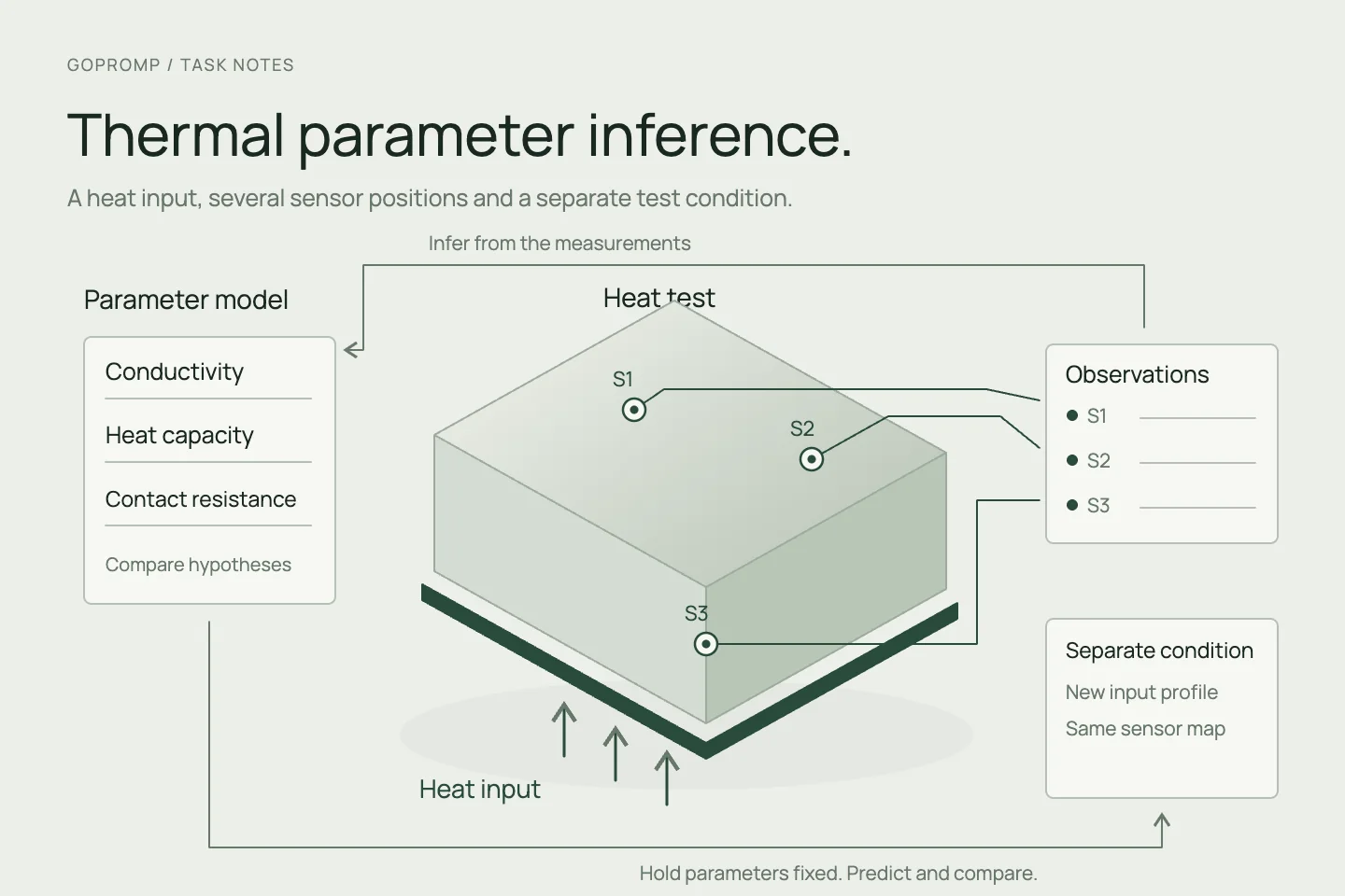
When a heater warms more slowly than expected, the cause may be higher heat capacity, stronger heat loss or less power actually reaching the tested component. A close fit to one temperature curve may not distinguish these explanations. Engineers need to know which parameters the available records can identify, whether the model supports the next power adjustment and which measurement is still missing.
We organise a parameter-inference round around known heating inputs and temperature time series from multiple locations. Start with a thermal model appropriate to the task, compare parameters, plan experiments and check new conditions. Give engineers the estimates together with explanations not yet ruled out, rather than only a curve fitted to measurements.
Which decision must the model support?
For predicting warm-up time, a small number of thermal nodes can represent energy exchange between heater, heated component and environment. Heat capacity describes storage, heat-transfer coefficients or conductances describe exchange, and contact parameters describe resistance at joints. If sensors show substantial spatial differences, assess the need for more nodes or spatial solving; do not begin with every material and interface parameter unknown.
The forward problem calculates sensor temperatures from given parameters, inputs and initial states. The inverse problem searches for parameters that explain measurements. Every parameter comparison should use the same forward calculation, retaining geometry, units, material versions and boundary assumptions.
The heating input should be measured and aligned in time with temperature records. A power-supply setting is not necessarily the heat reaching the component; wires, supports and housings can carry heat away. Unknown input efficiency can remain an open question, but freely adjusting it alongside all thermal parameters does not establish intrinsic material properties.
One curve can have several explanations
For a simple thermal node, cooling speed depends on the ratio of conductance to heat capacity. With only a single sensor’s temperature trace after heating stops, the two may compensate and produce similar curves. Reliable heating power, near-equilibrium temperature differences and the heating transient provide different information, although complex connections may leave other ambiguities.
First examine the model structure and observables: which parameters cannot be identified separately even with ideal data, and which are theoretically distinguishable but hard to estimate given current noise, duration and sensor positions? The former needs different measurements or parameterisation; the latter needs more informative experiments. A different optimiser does not automatically solve either problem.
For example, explanation A uses greater heat capacity and stronger heat loss; B uses lower capacity and weaker loss. Both fit the existing cooling phase but predict different responses to a new heating pulse. Retaining both explanations and their parameter relationships is more useful than selecting the lowest-loss set. If only a parameter combination is identifiable, report that combination rather than inventing separate precise values.
Choose experiments and sensors around the unknowns
The next input should distinguish A from B. Within an approved operating range, compare heating and cooling intervals of different durations so storage, contact heat transfer and environmental loss appear in different phases. Compare predicted temperature changes and measurement noise with the candidate models, then have the experimental team choose an executable input. Avoid another experiment confined to the region where both explanations agree.
More sensors are not automatically better. Positions near the heater, on either side of a contact and on distant components may inform different unknowns. Consider installation disturbance to heat paths, response speed and repeatable positioning. If existing sensors cannot resolve interface temperature differences, add measurements rather than asking the model to infer every contact parameter from distant temperatures.
For each round, record actual power, ambient and initial temperatures, installation state and sensor calibration. If the intended excitation was not completed—for example, because of a power limit or early stop—label the actual conditions first. Only data usable with the actual input enters inference; an interrupted run is not a new material response.
From physics solves to parameter search
Start with constrained parameter optimisation: each parameter set drives the physical solver, prediction–measurement differences are calculated, then another set is proposed. Heat capacity and heat-transfer parameters remain in physically permissible ranges. Solver failures, abnormal energy balances and excessive numerical error are not valid candidates. Comparing temperature trajectories is usually safer than differentiating noisy temperatures directly.
The objective should account for sensor errors, temporal correlation and anomalous records, so a high-frequency sensor does not dominate merely through sample count. Priors may come from material information, independent measurements or approved parameter ranges, but report sensitivity to them. A narrow interval imposed by a strong prior does not mean the data sufficiently identified the parameter.
Search from multiple initial values, then examine whether other parameters can compensate when one changes. If computation is expensive, train a surrogate to screen parameter regions and return key comparisons to the physical solver. Neural models can learn unknown heat-transfer terms within a defined range but do not replace identifiability checks. A small physics-constrained loss proves neither parameter uniqueness nor accuracy under new conditions. Language models help organise configurations and records; they do not invent thermal parameters from text.
Calibration records are not final proof
Separate complete experiments used for fitting from experiments used for evaluation. Randomly splitting adjacent times on one heating curve tests nearby interpolation in the same process, not independent validation. Hold out complete input sequences or operating conditions and inspect trajectories, peaks and response times using measures tied to the model’s actual purpose.
Look beyond mean error: does the prediction range accommodate plausible measurement variation, and do errors concentrate during startup, near contacts or at high temperatures? Discuss measurement uncertainty, parameter uncertainty and model omissions separately rather than folding every discrepancy into one broad interval.
Before changing installation, cooling method or temperature range, determine whether the original parameters still mean the same thing. An effective heat-transfer parameter estimated for one installation may combine several heat paths; it is not automatically an invariant material constant on another device. New conditions need their own checks. Successful calibration has not validated them.
Use residuals to decide what to measure or remodel
If several parameter sets explain current records but disagree on the next decision, prioritise an input or sensor position that distinguishes them. If different starting values produce the same local residual—for example, consistently early heating on one side of an interface—check synchronisation, sensor delay and installation before considering missing thermal nodes or temperature dependence. Do not simply keep widening parameter ranges.
If the heating input was not executed, revise the experiment record or execution conditions. If information is insufficient, add measurements. Change equations and parameterisation only after finding the model assumptions unsuitable. Retain the reason for each change, rerun affected calculations and keep new calibration separate from the next independent evaluation.
Delivery includes a versioned forward problem, parameter definitions and constraints, raw input and temperature records, optimisation settings, candidate explanations and complete operating-condition checks. A user should be able to revisit an estimate, identify its input dependencies and unresolved parameter ambiguities, and understand why the next experiment was chosen. Parameter inference then supports the next R&D decision rather than merely making a fitted curve look better.